Load Flow Study, Explained

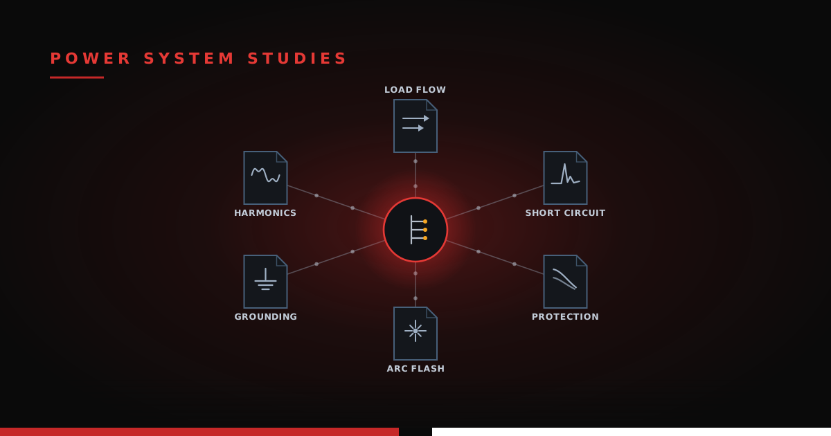
The load flow study is the first real study on a solar or storage project, and the one everything else leans on. In our overview of the studies, it sits at the root of the tree; short circuit, protection, and arc flash all inherit numbers that start here.

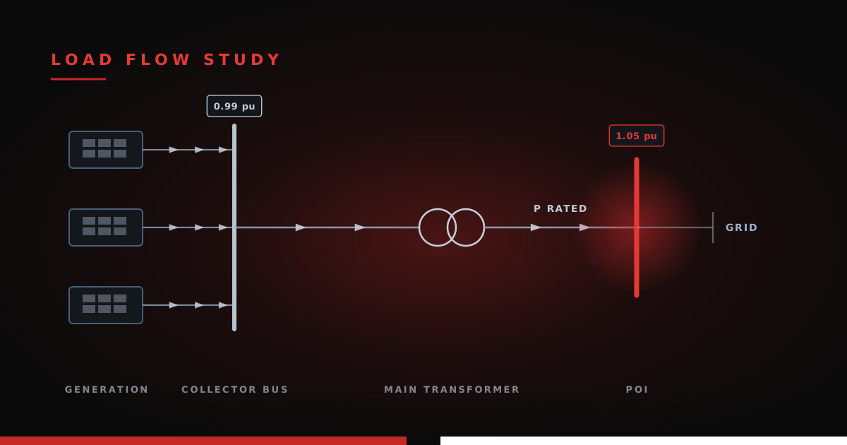
Stripped down, the load flow study answers one question: can this plant actually push its rated megawatts onto the grid while holding voltage and reactive power where the utility demands, without cooking a transformer or dragging a bus out of its voltage band? The one-line says the plant should work. The load flow study is how you prove it does, at a specific site, tied to a specific grid.

That last part is why you cannot dust off the last project's answer. Same plant, different point of interconnection, different grid strength standing behind it, and the numbers move.

WHY THE STUDY EXISTS

A load flow study is the steady-state picture of the plant: a single frozen moment with the plant running, showing how much real and reactive power flows through every conductor and transformer, what the voltage is at every bus, and whether anything is over its rating or outside its allowed voltage band.

That picture does a lot of work. It proves the plant can deliver its contracted real power to the point of interconnection while keeping voltage in band. It catches the quiet failures: a collector feeder loaded past its ampacity, a main transformer running hot, losses eating into the plant's output, a bus sagging below limits on a heavy day. It is also where reactive-support hardware gets sized (the capacitor banks and reactors on the one-line) and where transformer tap settings get chosen.

And it is where a specific federal requirement becomes a real number. FERC Order 827 requires every newly interconnecting solar, wind, or storage plant to provide reactive power across a power factor range of 0.95 leading to 0.95 lagging, at all output levels above zero, measured at the high side of the collector substation transformer. That single rule is the reason half of the study's work exists, and we will come back to it.

THE SOFTWARE, AND WHY

You do not run a real load flow study by hand. A utility-scale plant plus the grid it ties into is thousands of buses, and the equations are nonlinear, so the whole thing is solved iteratively by a computer.

For the interconnection study, the tool is almost always Siemens PSS/E. The reason is practical: the utility models the surrounding transmission system and hands you that model as a PSS/E "base case." You drop your plant into their case and study its effect at the point of interconnection, in the context of the real grid around it. Try to do that in a different tool and you are fighting the file format before you have solved anything.

The plant-internal study, the one that checks your collector feeders and pad-mount transformers, is often run in ETAP or DIgSILENT PowerFactory, which model the medium-voltage system in more native detail. Underneath all of them is the same engine: a Newton-Raphson solver, iterating toward a voltage solution that balances power at every bus.

WHAT IT SOLVES FOR

Here is the core of it. At every bus in the system, the study is solving for two unknowns: the voltage magnitude and its phase angle. It knows how much real power (P) and reactive power (Q) are being injected or drawn at each bus, and from those it has to find the voltages that make the whole network balance.

The relationship it enforces at each bus looks like this:

P_i = V_i · Σ V_k · (G_ik·cos θ_ik + B_ik·sin θ_ik)

with a matching equation for the reactive power Q. In plain terms, the power flowing into a bus depends on its own voltage, the voltages of every bus it connects to, the angle differences between them, and the impedance of the lines in between. You will notice that voltages multiply with voltages and the angles sit inside sines and cosines - there is no clean algebraic answer. Newton-Raphson handles it by guessing a solution, measuring how far off the power balance is, and using the slope of the equations (the Jacobian) to take a smarter guess, over and over until it converges (iterative method). That loop is why it is a computer's job, it can compute thousands of iterations with ease.

Side note: In the power systems class I took in college, we were required to do three iterations by hand. It took a whole afternoon.

Solving the network once is only half of it. The real work is proving the plant holds up across the operating envelope the utility requires. You run the plant at full real output and sweep it through a grid of conditions:

• Power factor: 0.95 lagging, unity, and 0.95 leading
• POI voltage: 0.95, 1.0, and 1.05 per unit

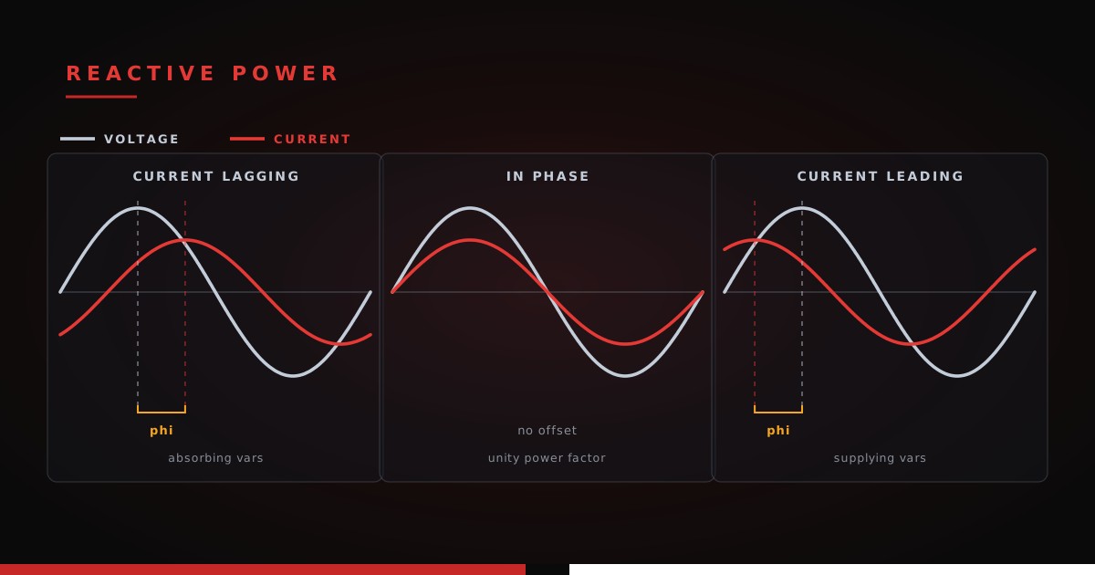
That is a three-by-three matrix of nine corners, and it is exactly the FERC Order 827 envelope. The two power-factor extremes are the interesting ones. At 0.95 lagging the plant supplies reactive power, propping voltage up, which is what a weak grid needs on a heavy day. At 0.95 leading the plant absorbs reactive power, pulling voltage down, which is what a stiff grid needs when voltage runs high. Unity is the easy middle. The plant has to hold every one of those corners, at each voltage, without exceeding an equipment limit.

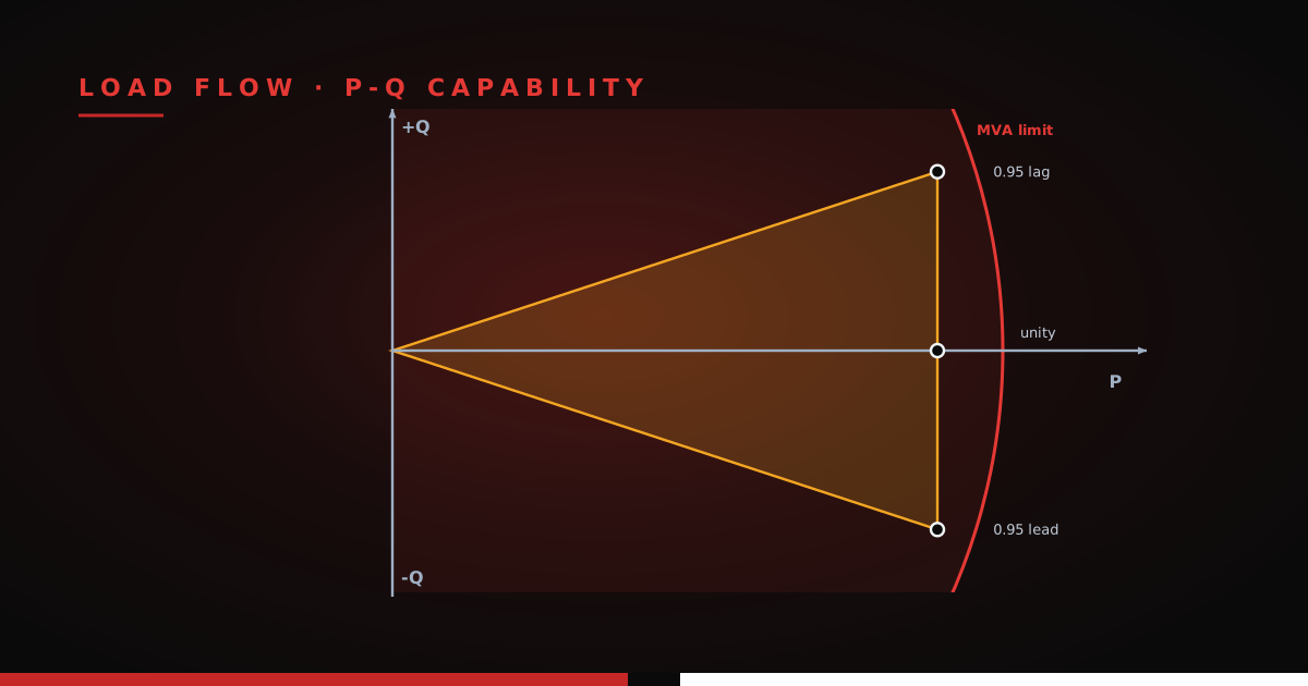
That whole envelope is what a P-Q capability curve draws. Since the 0.95 power factor limit is proportional to real output, the required reactive power grows with P. At rated output the plant owes about 0.33 MVAr for every MW. Plot the requirement across the full range of P and you get a wedge that opens to the right, not a box. Lay that wedge against the curve of what the inverters can deliver, and if the capability contains the wedge, the plant passes.

THE OUTCOMES

A load flow study ends in one of three places.

It passes. The plant delivers rated real power to the POI and holds the required reactive envelope at every voltage, with every conductor, transformer, and bus inside its limits. Nothing to fix; the design as drawn works for this site.

It fails on real power. The plant cannot get its full megawatts to the point of interconnection. Usually this is a thermal or voltage-drop problem: a collector feeder or the main transformer overloads, or the losses and voltage drop across a long gen-tie are large enough that the plant runs out of headroom before it hits rated output. The fixes are physical: upsize the conductors (the same tradeoff our voltage drop calculator runs on a single circuit), pick a larger transformer, adjust the tap settings, or in the worst case trim the plant's rating. This failure is less common on a well-sized collection system, but long or weak interconnections surface it.

It fails on reactive power. This is the common one. The inverters cannot supply or absorb enough reactive power to hold the required power factor at the voltage extremes. The trap is that an inverter's reactive capability shrinks as its real-power output rises, because it is bounded by a fixed MVA rating; at full real output there may not be enough headroom left to reach 0.95 at the far corners. The fixes are the reactive hardware the study exists to size: capacitor banks to supply vars, reactors to absorb them, or a STATCOM for fast dynamic support. Add the hardware, re-run, and confirm the capability curve now swallows the required wedge.

And that re-run matters, because the load flow study is a loop, not a single pass. Change a conductor size, add a capacitor bank, or move a tap, and the voltages and flows shift everywhere. You solve it, read the result, adjust, and solve again until the plant clears the whole envelope.

A NOTE FOR STORAGE

A battery plant makes the study bigger, because it has more states than a solar plant. You run it at full discharge and at full charge, since the real power flows both directions and each direction stresses the system differently. You also check it across the plant's life, because as the battery is augmented and its internal impedances shift, the reactive picture at the POI moves with it. More operating points, same envelope to hold.

WHERE IT LEADS

The load flow study gives you a plant that can deliver its power and hold its voltage on a normal day. What it does not tell you is what happens when something breaks. For that you need the fault currents, which is the next study in the stack: short circuit. That one takes the network model you just built and asks how much current shows up when a fault hits, and it is where the ratings on every breaker and cable come from.