Understanding Load Factor for Solar + BESS Underground Cable Ampacity

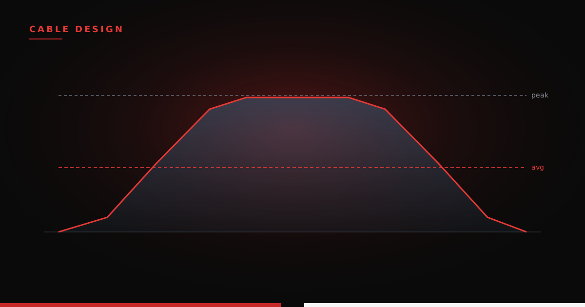
Load factor is one of those terms everyone nods along to and few actually pin down — and it gets misunderstood about as often by engineers as by the people who hire them. On solar and battery storage sites alike, one of the most useful places it shows up is underground medium-voltage cable ampacity. Used well, it right-sizes the collection and gen-tie cable and saves real copper. Used carelessly, it buries an undersized conductor that's almost impossible to get back. The mechanism is the same for both technologies; what differs is the load profile that drives it.

START WITH THE LOAD PROFILE

Underground cable ampacity is a heat-transfer problem. The conductor can only run so hot — 90°C for typical XLPE — and everything comes down to moving that heat out through the insulation, any duct, and the surrounding soil. The soil is usually the bottleneck, and it has thermal inertia. The soil pressed right against the cable heats and cools quickly as the load changes. The bulk of the soil farther out — the far field, the ground beyond the cable's immediate surroundings — is slow to respond, and it settles toward the average heat over a day rather than the moment-to-moment peak. So a cable that runs hard for only part of the day warms that far-field soil less than one loaded around the clock, and that difference is the whole basis for a load-factor credit.

A baseline thermal study assumes the worst case — continuous loading, 100% of the time. Backing off that assumption to the site's real duty is where the ampacity headroom comes from, so the load profile fed into the study matters. And this is where solar and BESS diverge:

• Solar output follows the sun: zero overnight, a morning ramp, a midday peak, and an evening ramp back down. How long it holds that peak depends on the site. In a cloudier region or at a modest DC/AC ratio the curve is peaky and the load factor is low; in a very sunny region at a high DC/AC ratio the inverters clip to a long midday plateau that holds near peak for much of the day, driving the load factor up. Either way, modeling the real profile — if the software supports it — is what captures the true credit instead of guessing at it.
• BESS is blockier. The worst-case bounding profile is simple: a full discharge running straight into a full charge, back to back — a rectangular block at peak current for the cycle, and zero the rest of the day. That simplicity is a feature; the bounding case is easy to define and hard to argue with.

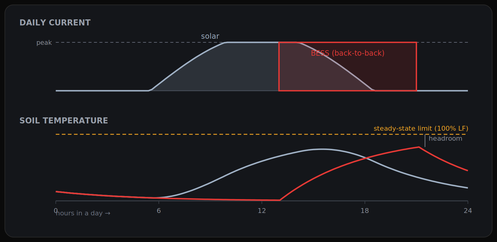
That back-to-back square wave is the worst-case bound, but it's highly unlikely to actually happen. It would require the grid conditions demanding a full discharge to resolve at the exact moment the last kilowatt-hour leaves the battery, and then immediately flip to conditions that support a full charge. Full-discharge events usually come from outages, which rarely clear that cleanly or that fast. Real duty is gentler: a common role is balancing solar — charging midday when energy is abundant and discharging into the morning and evening peaks — a smoother profile than the square wave assumed here. The square wave stays useful precisely because it's conservative: if the cable survives it, it survives anything the battery realistically does. And because even that real duty leaves the cable idle for meaningful stretches, the load-factor credit is genuine for BESS too, not just solar.

LOAD FACTOR VS. LOSS FACTOR

There's a distinction buried in that "average heat" idea that trips up a lot of otherwise-careful studies.

Load factor is the average load divided by the peak load over a chosen period — 24 hours, for Neher-McGrath. It's a ratio of currents, and by definition it always lands between 0 and 1: there is no such thing as a negative load factor, and nothing above 1.

But cable heating scales with I²R, so what actually drives the soil temperature is the average of the losses, not the average of the current. That's the loss factor (or loss load factor): average losses ÷ peak losses. Because losses go as current squared, the loss factor is always less than or equal to the load factor, and the gap depends on the profile shape:

• For an ideal on/off duty — full current or nothing, which is exactly the BESS bounding case — the two are identical. During the on-hours the losses are at peak; during the off-hours they're zero; so the loss factor equals the fraction of time on, which is the load factor. For BESS's simple envelope, there's nothing to convert.
• For a smoothly varying profile — a solar plant ramping to a midday plateau and back — the loss factor sits below the load factor, because the hours spent at partial output contribute disproportionately little heat.

When only the load factor is on hand, a common empirical bridge is:

LLF ≈ 0.3 · LF + 0.7 · LF²

The coefficients vary by system (0.15/0.85 and 0.2/0.8 show up too), but the shape is always the same: a blend of the load factor and its square.

The practical upshot: Neher-McGrath's earth term uses the loss factor. Feed it the raw current load factor for a solar profile and the average heating is overstated — conservative, but it leaves ampacity on the table. Convert to the loss factor to claim the real credit. For BESS on/off duty, the two are equal, so it's moot.

THE MATH: WHERE IT ENTERS NEHER-MCGRATH

Strip Neher-McGrath down to its bones and cable ampacity is just thermal Ohm's law — the allowable conductor temperature rise divided by the resistance the heat has to climb through to reach the ambient soil:

I = √( ΔΘ / ( Rac · Rθ ) )

ΔΘ is the allowable rise (a 90°C conductor in 20°C earth gives 70°C), Rac is the conductor's AC resistance, and Rθ is the total thermal resistance from conductor to ambient.

The loss factor doesn't touch the conductor or the insulation — it lives in the earth portion of Rθ. Neher-McGrath splits the surrounding soil at a characteristic diameter Dx (how deep the daily heating wave reaches — on the order of 200 mm in typical soil, and a function of the soil's thermal diffusivity):

Rearth = (ρ / 2π) · [ ln(Dx / De)  +  LLF · ln(4L / Dx) ]

• Inside Dx, near the cable, the soil tracks the peak heat — the ln(Dx/De) term gets no relief.
• Outside Dx, in the far field, the soil tracks the average heat — so the ln(4L/Dx) term is scaled by the loss factor.

Drop the loss factor below 1 and that second term shrinks, Rearth falls, and the allowable current climbs. Put numbers on it, using the BESS bounding case where the loss factor equals the load factor at 0.33 — soil resistivity ρ = 0.9 K·m/W, 0.9 m of cover, a 50 mm cable, Dx ≈ 210 mm:

• Continuous (LLF = 1.0): Rearth ≈ 0.61 K·m/W
• Once-daily cycle (LLF = 0.33): Rearth ≈ 0.34 K·m/W

The earth resistance drops by roughly 45%. Carry that back through the equation — with the cable's internal resistances adding, say, another 0.4 K·m/W — and Rθ falls from about 1.0 to 0.74. Because current scales with 1 / √Rθ, that works out to √(1.0 / 0.74) ≈ a 17% bump in ampacity, often exactly enough to drop a conductor size.

That's the credit in one number. Two caveats before spending it: this is the stripped-down version — a real study keeps the dielectric loss, the sheath and armor loss factors, and the mutual heating from every other cable in the bank, which is why it belongs in software (ETAP, CYMCAP, Cableizer) rather than on a napkin. And it rides entirely on the soil resistivity ρ — more on that below.

KEEP A FLOOR AT 0.5

Here's where judgment comes in, and where good practice deviates from what the pure math would allow. Even when a single daily cycle pencils out to a 0.33, it's worth holding the modeled load factor to a floor — and 0.5 is a reasonable one. There's no code behind the number; it's a buffer, and it covers three things a clean 24-hour calc doesn't:

• Abnormal soil conditions. The study is only as good as the resistivity and moisture assumed for it. A dry pocket, a stretch of poor backfill, or seasonal drying can push the local resistivity well above the design value. Extra load-factor margin absorbs some of that.
• Abnormally hot summers. A run of hot days with warm nights means the soil doesn't cool overnight the way an average design year assumes. The daily "reset" the calc counts on gets weaker exactly when the cable is working hardest.
• Use-case variability. MV cable goes in the ground for thirty-plus years, and the duty it sees can grow. On top of the base charge/discharge cycle, a battery may pick up roles no one planned for — fast frequency response, spinning reserve, standby backup for a wind plant — each stacking extra current onto the profile the design assumed. Added to a full cycle, they put more heat into the ground and effectively shorten the soil's cooling window. A floor leaves room for duties the cable wasn't originally sized around.

Below 0.5, all three of those margins get thin at once. So 0.5 isn't physics — it's a hedge against a thirty-year asset outliving the assumptions it was sized on.

CHECK FOR SLOW THERMAL RUNAWAY

Neher-McGrath only requires a 24-hour cyclic calculation, and that's fine as long as each day fully resets — the soil sheds the day's heat overnight and starts the next morning cool. But that assumption can quietly fail, and a single-day calc is blind to it.

In the hottest month, across a run of hot days and warm nights, the soil may not shed all of one day's heat before the next day's load piles more on. Day over day, the baseline soil temperature creeps upward. A calc that showed the peak comfortably under the limit can miss a slow, cumulative climb that eventually crosses it — a thermal runaway that only reveals itself over weeks.

If the software supports it, run a transient thermal study across the hottest month the site will actually see, with realistic ambient and soil boundary conditions. It answers the question a 24-hour calc can't: does nightly cooling truly offset daytime heating, or does the soil charge up over weeks to a steady state hotter than any single day predicted?

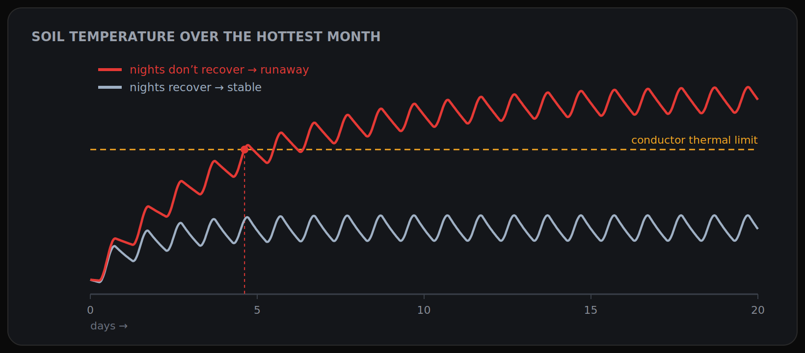
This is also where the load-factor floor earns its keep a second time. The margin from not dropping below 0.5 is precisely the cushion that keeps a hot-month soil-charging trend from tipping into an exceedance.

THE STUDY IS ONLY AS GOOD AS THE SOIL

Every number above rests on one input more than any other: the soil's thermal resistivity. Get it wrong and no amount of careful load-factor work will save the result — a bad resistivity value swamps the load-factor credit several times over. Load factor is a fine-tuning lever; resistivity is the foundation the whole study stands on. That means proper thermal resistivity testing, backed by engineered thermal backfill where the native soil falls short. It's a big enough topic to deserve its own treatment, and we plan to cover it in a future post — but the short version is simple: no load-factor credit is worth more than the resistivity it's built on.

KEY TAKEAWAYS

• Load factor lets a cyclic load carry more current than a continuous one, because the far-field soil responds to average heat, not peak — a real credit on both solar and BESS sites.
• Solar rewards a realistic profile; BESS rewards a simple bounding one. Solar's shape varies with the site and is worth modeling honestly; BESS's worst case is a back-to-back cycle that's easy to define — and still worth crediting.
• Use the loss factor, not the raw load factor, in the Neher-McGrath earth term. They're equal for BESS on/off duty; for solar, LLF ≈ 0.3·LF + 0.7·LF² and sits below the load factor.
• Keep a floor around 0.5 — the buffer covers abnormal soil, hot summers with poor overnight cooling, and added duties the cable wasn't sized for.
• Run a transient study over the hottest month if the software allows, to catch a slow thermal runaway a 24-hour calc can't see.
• It all rides on the soil. Thermal resistivity swings ampacity far more than load factor — get the testing right first.